Recommender System using Content Filtering
Data wrangling, feature construction, and similarity-based recommendations on TMDB5000.
Introduction
What are Recommendations Systems? Strictly speaking, Recommendations Systems (or RecSys as they are usually abbreviated) are a class of information filtering systems. Their goal is to improve the quality of results being delivered to the end user, by taking into account different heuristics related to the user itself.
Recommendation Systems power nearly every kind of content on the Internet, from search results on your favorite search engine to the Customers Who Bought This Item Also Bought window on Amazon.com. Netflix uses recommender systems to help you find the next show or movie to watch. They're everywhere and highly effective because of their ability to narrow down content for a user, be it a movie to watch or an item to buy.
There are primarily three different kinds of RecSys, each of which is formulated differently and has different operating characteristics.
- Demographic
Demographic(or popularity) based RecSys offer generalized recommendations. They offer non-personalized recommendations, instead focusing on what's universally popular(within the problem domain) and assuming that generality holds for all users from the target demography. They are simple and easy to get started with and don't require any kind of user data to be effective. That said, they're not as effective as others types of RecSys that we'll look at.
- Content Based Filtering
Classification based RecSys try to group together similar items. If a user has seen or shopped from an item, they're more likely to be interested in other entities from the same bucket. Instead of relying on user information, they rely on information about the item itself to group similar items together in the same bucket. More information can be found here
- Collaborative Filtering
Collaborative Filtering adds to the idea of Content Based Filtering by using similarities between user data and item data to make recommendations. To put it simply, consider the following scenario: person A has seen movie X and person B has seen movie Y. Now, it turns out person A and B have similar tastes. So the system will then recommend movie Y to A accounting for that similarity. More information can be found here on the Google Developers blog
TMDB5000 Dataset
TMDB5000 is a Kaggle hosted database derived from the TMDB API. You can learn more about TMDB on their website. It consists of roughly 5000 data entries, each of which has 20 features that we can work with. The data has probably gone through some amount of pre-processing steps, though there's a lot to be done, as we'll see below.
Let's dive into some of the code, so we can get started.
Note: This project was written as part of a challenge submission for the Insight Data Science Fellowship interview. As such, it focuses on breadth rather than depth. A more in depth post, building on this, will follow soon.
#hide
#magic commands
%matplotlib inline
%reload_ext autoreload
%autoreload 2
#collapse-hide
#imports

from utils import build_word_cloud, clean_num, get_month, get_day, get_director, get_list, clean_list, create_feature
from pathlib import Path
import warnings
warnings.simplefilter('ignore')
import ast
import math
import datetime

import pandas as pd
import matplotlib.pyplot as plt
import seaborn as sns

from sklearn.feature_extraction.text import TfidfVectorizer, CountVectorizer
from sklearn.metrics.pairwise import cosine_similarity
dataPath = Path('data/')
movies = pd.read_csv(dataPath/'tmdb_5000_movies.csv')
credits = pd.read_csv(dataPath/'tmdb_5000_credits.csv')
movies.shape
(4803, 20)
movies.info()
<class 'pandas.core.frame.DataFrame'>
RangeIndex: 4803 entries, 0 to 4802
Data columns (total 20 columns):
 #   Column                Non-Null Count  Dtype
---  ------                --------------  -----
 0   budget                4803 non-null   int64
 1   genres                4803 non-null   object
 2   homepage              1712 non-null   object
 3   id                    4803 non-null   int64
 4   keywords              4803 non-null   object
 5   original_language     4803 non-null   object
 6   original_title        4803 non-null   object
 7   overview              4800 non-null   object
 8   popularity            4803 non-null   float64
 9   production_companies  4803 non-null   object
 10  production_countries  4803 non-null   object
 11  release_date          4802 non-null   object
 12  revenue               4803 non-null   int64
 13  runtime               4801 non-null   float64
 14  spoken_languages      4803 non-null   object
 15  status                4803 non-null   object
 16  tagline               3959 non-null   object
 17  title                 4803 non-null   object
 18  vote_average          4803 non-null   float64
 19  vote_count            4803 non-null   int64
dtypes: float64(3), int64(4), object(13)
memory usage: 750.6+ KB
We can see that we have data on 4803 different movies. The different features available include the budget, revenue of the movie, cast and crew as well as descriptive informatin about the genres and keywords.
Let's look at a few samples of the data, so we can get a sense of the work that we have to do before we can start extracting meaningful information.
movies.head(2)
budget                                             genres  \
0  237000000  [{"id": 28, "name": "Action"}, {"id": 12, "nam...
1  300000000  [{"id": 12, "name": "Adventure"}, {"id": 14, "...

                                       homepage     id  \
0                   http://www.avatarmovie.com/  19995
1  http://disney.go.com/disneypictures/pirates/    285

                                            keywords original_language  \
0  [{"id": 1463, "name": "culture clash"}, {"id":...                en
1  [{"id": 270, "name": "ocean"}, {"id": 726, "na...                en

                             original_title  \
0                                    Avatar
1  Pirates of the Caribbean: At World's End

                                            overview  popularity  \
0  In the 22nd century, a paraplegic Marine is di...  150.437577
1  Captain Barbossa, long believed to be dead, ha...  139.082615

                                production_companies  \
0  [{"name": "Ingenious Film Partners", "id": 289...
1  [{"name": "Walt Disney Pictures", "id": 2}, {"...

                                production_countries release_date     revenue  \
0  [{"iso_3166_1": "US", "name": "United States o...   2009-12-10  2787965087
1  [{"iso_3166_1": "US", "name": "United States o...   2007-05-19   961000000

   runtime                                   spoken_languages    status  \
0    162.0  [{"iso_639_1": "en", "name": "English"}, {"iso...  Released
1    169.0           [{"iso_639_1": "en", "name": "English"}]  Released

                                          tagline  \
0                     Enter the World of Pandora.
1  At the end of the world, the adventure begins.

                                      title  vote_average  vote_count
0                                    Avatar           7.2       11800
1  Pirates of the Caribbean: At World's End           6.9        4500
Data Wrangling
As can be seen above, several features are in a stringified format, so we'll need to convert those back to their original formats. There's a homepage feature which has no information present for a majority of the data points, so removing that feature shouldn't lead to any major data loss.
Almost all of the features are represented as generic object dtypes, rather than native data types, so we'll look into that as well. We already have certain features, namely vote_count and vote_average that we can use to gain some kind of insight and build a baseline recommendation system.
Removing original_title feature
We have two features related to the title/name in the movie, namely title and original_title. There are however, a small number of cases when those two features aren't exactly the same (~6%) of the total dataset. A visual inspection tells us even in those cases, we can get the name of the movie by looking at title and original_language features.
Considering we're trying to build a recommender system, the name of the movie is going to be one of the lesser significant features and we can safely remove it from consideration.
cols = ['title', 'original_title', 'original_language']
movies[movies['original_title'] != movies['title']][cols].head()
title                original_title  \
97                            Shin Godzilla                        シン・ゴジラ
215  Fantastic 4: Rise of the Silver Surfer  4: Rise of the Silver Surfer
235            Asterix at the Olympic Games   Astérix aux Jeux Olympiques
317                      The Flowers of War                         金陵十三釵
474                               Evolution                     Évolution

    original_language
97                 ja
215                en
235                fr
317                zh
474                fr
movies = movies.drop('original_title', axis = 1)
Sanitizing the revenue feature
movies['revenue'].describe()
count    4.803000e+03
mean     8.226064e+07
std      1.628571e+08
min      0.000000e+00
25%      0.000000e+00
50%      1.917000e+07
75%      9.291719e+07
max      2.787965e+09
Name: revenue, dtype: float64
print(movies[movies['revenue'] == 0].shape[0]/(movies.shape[0]))
0.29710597543202166
We can see above that roughly 30% of the entries in our data have no revenue ie revenue is 0. While it may come across as a not so useful feature, we can use it later. For now, let's sanitize the zero values so we get some info out of it.
movies['revenue'] = movies['revenue'].replace(0, math.nan)
Sanitizing the budget feature
movies['budget'].describe()
count    4.803000e+03
mean     2.904504e+07
std      4.072239e+07
min      0.000000e+00
25%      7.900000e+05
50%      1.500000e+07
75%      4.000000e+07
max      3.800000e+08
Name: budget, dtype: float64
print(movies[movies['budget'] == 0].shape[0]/(movies.shape[0]))
0.21590672496356444
We can see above that roughly 22% of the entries in our data have no budget ie budget is 0. Let's sanitize the zero values, so we can use it later.
movies['budget'] = movies['budget'].replace(0, math.nan)
Sanitizing year feature
Let's sanitize the year column. Currently it's a generic object datatype, we'll convert it to a datetime representation
movies['year'] = pd.to_datetime(movies['release_date'], errors='coerce').apply(\
                lambda x: str(x).split('-')[0] if x != math.nan else math.nan)
Create new feature: return
The feature return will describe the Return On Investment(ROI) for a movie. It's simply a numeric value that describes the revenue in terms of multiples from the original budget (investment).
movies['return'] = movies['revenue'] / movies['budget']
movies['return'].describe()
count    3.229000e+03
mean     2.954822e+03
std      1.506101e+05
min      5.217391e-07
25%      1.022463e+00
50%      2.300366e+00
75%      4.420822e+00
max      8.500000e+06
Name: return, dtype: float64
There's a lot more cleaning and aggregation that needs to be done. But without exploring the data first, and getting some kind of intuition for the data, we don't really know what to do. We'll explore the data first, and do any kind of cleaning and generating features on the fly later as needed.
EDA
Let's move on to do some exploratory data analysis, where we'll explore the dataset.
Word Clouds
We start by building world clouds, to get an idea of the titles and keywords for the dataset.
movies['title'] = movies['title'].astype('str')
movies['overview'] = movies['overview'].astype('str')
build_word_cloud(movies, 'title')

build_word_cloud(movies, 'overview')

Languages
Let's look into the different languages of the movies available in the dataset. If I could take a guess, just from looking at the data, I'd say most of the movies are in English, with a sprinking of some French, Japanese and Asian movies.
movies['original_language'].drop_duplicates().shape
(37,)
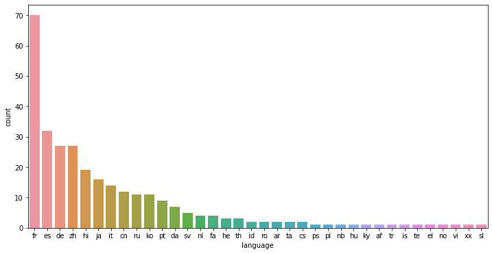
There are 37 different languages, that's a wide range. Let's plot the occurence of each language
languages = pd.DataFrame(movies['original_language'].value_counts())
languages['language'] = languages.index
columns = ['count', 'language']
languages.columns = columns
languages.head(7)
count language
en   4505       en
fr     70       fr
es     32       es
de     27       de
zh     27       zh
hi     19       hi
ja     16       ja
plt.figure(figsize=(10,5))
sns.barplot(x = 'language', y = 'count', data = languages)
plt.show()
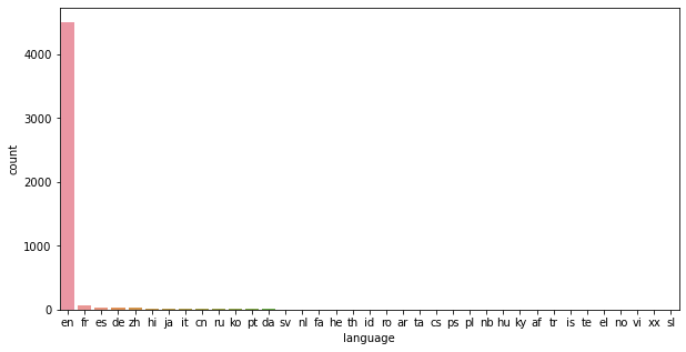
As expected, an overwhelmingly large number of the movies are in English. Let's look at a graph that makes it a bit easier for us to visualize the different languages present in the dataset.
plt.figure(figsize=(12,6))
sns.barplot(x = 'language', y = 'count', data = languages.iloc[1:])
plt.show()
Metrics
There are 3 fields in the dataset, which are hard metrics already given to us. They are popularity, vote_count and vote_average.
movies['popularity'] = movies['popularity'].apply(clean_num).astype('float')
movies['vote_count'] = movies['vote_count'].apply(clean_num).astype('float')
movies['vote_average'] = movies['vote_average'].apply(clean_num).astype('float')
#list movies by popularity
movies[['title', 'popularity']].sort_values('popularity', ascending = False).head(5)
title  popularity
546                  Minions  875.581305
95              Interstellar  724.247784
788                 Deadpool  514.569956
94   Guardians of the Galaxy  481.098624
127       Mad Max: Fury Road  434.278564
movies[['title', 'vote_count']].sort_values('vote_count', ascending = False).head(5)
title  vote_count
96         Inception       13752
65   The Dark Knight       12002
0             Avatar       11800
16      The Avengers       11776
788         Deadpool       10995
movies[['title', 'vote_average']].sort_values('vote_average', ascending = False).head(5)
title  vote_average
3519       Stiff Upper Lips          10.0
4247  Me You and Five Bucks          10.0
4045  Dancer, Texas Pop. 81          10.0
4662         Little Big Top          10.0
3992              Sardaarji           9.5
Release Dates
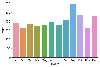
Amongst all the features, we could be looking at or creating, perhaps few are as important as time of release. When a movie is released tends to have a strong correlation with how well it does. Major franchisee movies tend to be released around the time of holidays/summer months. Conversely, movies released around the time of holidays go on to do a lot better than those released around the year. Let's try to plot this distribution
movies['day'] = movies['release_date'].apply(get_day)
movies['month'] = movies['release_date'].apply(get_month)
months = ['Jan', 'Feb', 'Mar', 'Apr', 'May', 'Jun', 'Jul', 'Aug', 'Sep', 'Oct', 'Nov', 'Dec']
sns.countplot(x = 'month', data = movies, order = months)
<matplotlib.axes._subplots.AxesSubplot at 0x196d5b41cc8>
print(movies['revenue'].mean())
117031352.91587678
The mean revenue for movies in our dataset is 82260638.65167603. Let's now try to plot only the release dates of the movies whose revenue is greater than the mean for the data.
means = pd.DataFrame(movies[movies['revenue'] > 82260638.65167603].groupby('month')['revenue'].mean())
means['month'] = means.index
plt.figure(figsize=(16,9))
plt.title('Average Revenue by Month')
sns.barplot(x = 'month', y = 'revenue', data = means, order = months)
<matplotlib.axes._subplots.AxesSubplot at 0x196d5b1f608>
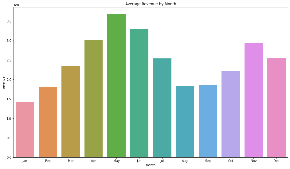
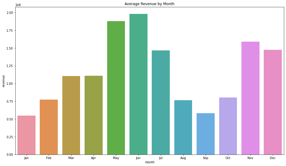
From the chart above, we can see that the summer months(April - June) have the most number of movies who fare better than the numerically average movie in the dataset.
How similar/dissimilar is this chart from one where we graph all movies against the mean revenue?
means = pd.DataFrame(movies[movies['revenue'] > 1].groupby('month')['revenue'].mean())
means['month'] = means.index
plt.figure(figsize=(16,9))
plt.title('Average Revenue by Month')
sns.barplot(x = 'month', y = 'revenue', data = means, order = months)
<matplotlib.axes._subplots.AxesSubplot at 0x196ddb37588>
Budget
Is there a correlation between the budget of a movie and its return?
plt.figure(figsize=(12,9))
sns.distplot(movies[movies['budget'].notnull()]['budget'])
<matplotlib.axes._subplots.AxesSubplot at 0x196d5f05588>
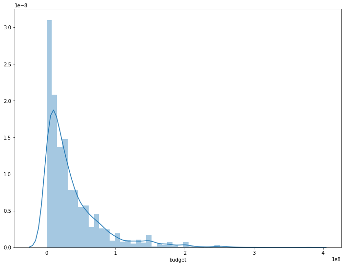
As we can see above, the budgets of the movies in the dataset are highly skewed , suggesting that a rather large number of movies have extremely small budgets
sns.jointplot(x = 'budget', y = 'revenue', data = movies)
<seaborn.axisgrid.JointGrid at 0x196db62a588>
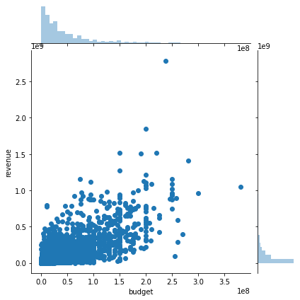
The graph above suggests that there's a strong correlation between the budget of a movie and its revenue.
Revenue
movies['revenue'].describe()
count    3.376000e+03
mean     1.170314e+08
std      1.834831e+08
min      5.000000e+00
25%      1.535290e+07
50%      5.175184e+07
75%      1.401651e+08
max      2.787965e+09
Name: revenue, dtype: float64
best_revenue = movies[['title', 'budget', 'revenue']].sort_values('revenue', ascending = False)
best_revenue
title       budget       revenue
0                        Avatar  237000000.0  2.787965e+09
25                      Titanic  200000000.0  1.845034e+09
16                 The Avengers  220000000.0  1.519558e+09
28               Jurassic World  150000000.0  1.513529e+09
44                    Furious 7  190000000.0  1.506249e+09
...                         ...          ...           ...
4797                     Cavite          NaN           NaN
4799                  Newlyweds       9000.0           NaN
4800  Signed, Sealed, Delivered          NaN           NaN
4801           Shanghai Calling          NaN           NaN
4802          My Date with Drew          NaN           NaN

[4803 rows x 3 columns]
A useful analysis that needs to be done here is to take inflation into account. The movies at the top are all from recent times, so maybe inflation analysis is something that's necessary to get meaningful information from this feature.
Genres
#convert string-ified lists to list representation
movies['genres'] = movies['genres'].fillna('[]').apply(
    ast.literal_eval).apply(lambda x: [i['name'] for i in x] if isinstance(x, list) else [])
series = movies.apply(lambda x: pd.Series(x['genres']),axis = 1).stack().reset_index(level = 1, drop = True)
series.name = 'genres'

genres = movies.drop('genres', axis = 1).join(series)
genres['genres'].value_counts().shape[0]
20
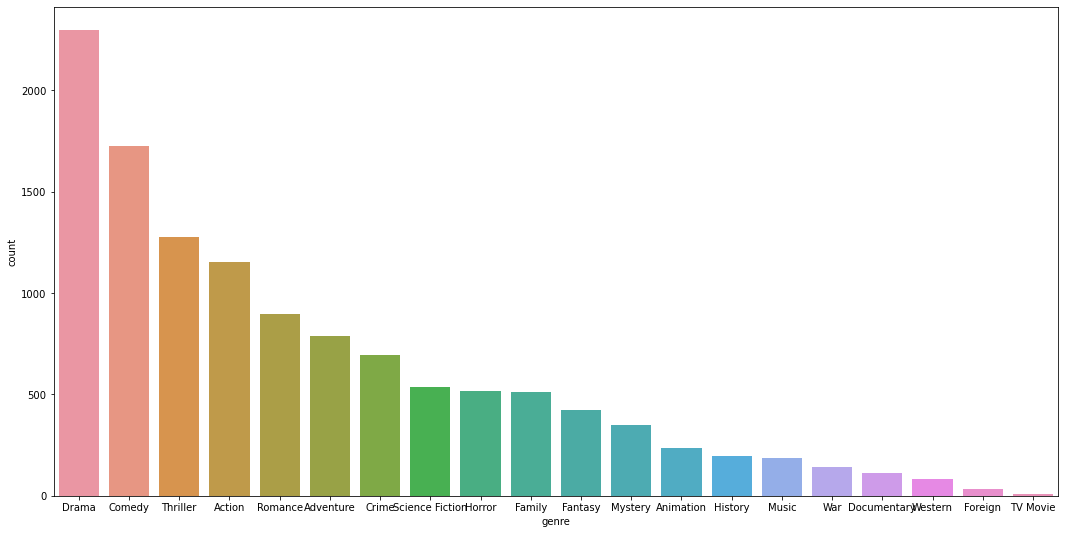
There are 20 different genres, which we look at below
popular = pd.DataFrame(genres['genres'].value_counts()).reset_index()
popular.columns = ['genre', 'count']
popular.head()
genre  count
0     Drama   2297
1    Comedy   1722
2  Thriller   1274
3    Action   1154
4   Romance    894
plt.figure(figsize = (18,9))
sns.barplot(x = 'genre', y = 'count', data = popular)
plt.show()
Let's look at the trends over time for a specific set of genres
genre = ['Drama', 'Action', 'Comedy', 'Thriller', 'Romance', 'Adventure', 'Horror', 'Family']
genres['year'] = genres['year'].replace('NaT', math.nan)
genres['year'] = genres['year'].apply(clean_num)
trends = genres[(genres['genres'].isin(genre)) & (genres['year'] >= 2000) & (genres['year'] <= 2016)]
ctab = pd.crosstab([trends['year']], trends['genres']).apply(lambda x: x/x.sum(), axis = 1)
ctab[genre].plot(kind = 'line', stacked = False, colormap = 'jet', figsize = (18,9))
plt.legend(bbox_to_anchor=(1, 1))
<matplotlib.legend.Legend at 0x196d65dca08>
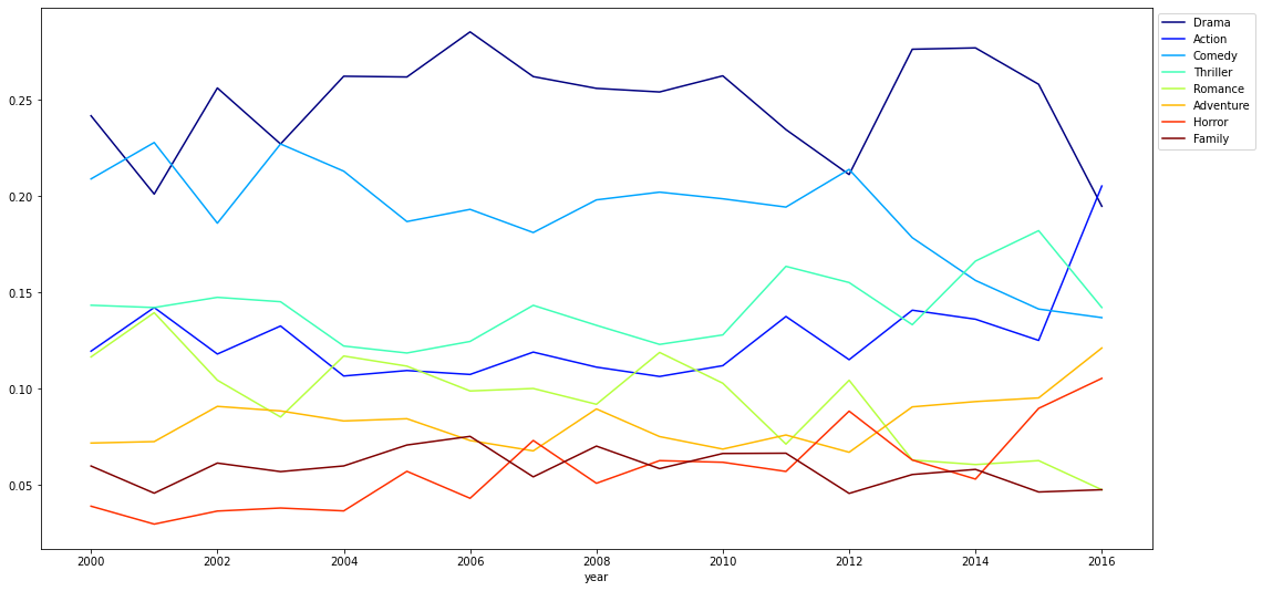
There seems to be a sharp decline in the number of drama movies from 2014-2016 while the number of movies under horror and action has gone up around the same time.
Modeling
There's a lot of interesting possibilities in terms of the viz that we could have done. Ideally, we will clean and analyze every possible feature and try to identify its importance towards the final task. However, for the purposes of keeping this clean and simple, I'll go ahead and build what we're actually here for: a recommendation system.
We'll be building a Content Filtering based RecSys. In a way, given the dataset, we are limited in terms of the approach we can take. We don't have user information available in the data, so collaborative filtering is unfortunately not an option. We do have metadata about the movies itself, and that fits in perfectly within the operating characteristics of a Content Filtering based recommendation system.
movies = pd.read_csv(dataPath/'tmdb_5000_movies.csv')
credits = pd.read_csv(dataPath/'tmdb_5000_credits.csv')
credits.head(2)
movie_id                                     title  \
0     19995                                    Avatar
1       285  Pirates of the Caribbean: At World's End

                                                cast  \
0  [{"cast_id": 242, "character": "Jake Sully", "...
1  [{"cast_id": 4, "character": "Captain Jack Spa...

                                                crew
0  [{"credit_id": "52fe48009251416c750aca23", "de...
1  [{"credit_id": "52fe4232c3a36847f800b579", "de...
movies.head(2)
budget                                             genres  \
0  237000000  [{"id": 28, "name": "Action"}, {"id": 12, "nam...
1  300000000  [{"id": 12, "name": "Adventure"}, {"id": 14, "...

                                       homepage     id  \
0                   http://www.avatarmovie.com/  19995
1  http://disney.go.com/disneypictures/pirates/    285

                                            keywords original_language  \
0  [{"id": 1463, "name": "culture clash"}, {"id":...                en
1  [{"id": 270, "name": "ocean"}, {"id": 726, "na...                en

                             original_title  \
0                                    Avatar
1  Pirates of the Caribbean: At World's End

                                            overview  popularity  \
0  In the 22nd century, a paraplegic Marine is di...  150.437577
1  Captain Barbossa, long believed to be dead, ha...  139.082615

                                production_companies  \
0  [{"name": "Ingenious Film Partners", "id": 289...
1  [{"name": "Walt Disney Pictures", "id": 2}, {"...

                                production_countries release_date     revenue  \
0  [{"iso_3166_1": "US", "name": "United States o...   2009-12-10  2787965087
1  [{"iso_3166_1": "US", "name": "United States o...   2007-05-19   961000000

   runtime                                   spoken_languages    status  \
0    162.0  [{"iso_639_1": "en", "name": "English"}, {"iso...  Released
1    169.0           [{"iso_639_1": "en", "name": "English"}]  Released

                                          tagline  \
0                     Enter the World of Pandora.
1  At the end of the world, the adventure begins.

                                      title  vote_average  vote_count
0                                    Avatar           7.2       11800
1  Pirates of the Caribbean: At World's End           6.9        4500
Join both the DataFrames on the id attribute, so we can incorporate features from both datasets.
credits.columns = ['id', 'title', 'cast', 'crew']
data = movies.merge(credits, on = 'id')
data.info()
<class 'pandas.core.frame.DataFrame'>
Int64Index: 4803 entries, 0 to 4802
Data columns (total 23 columns):
 #   Column                Non-Null Count  Dtype
---  ------                --------------  -----
 0   budget                4803 non-null   int64
 1   genres                4803 non-null   object
 2   homepage              1712 non-null   object
 3   id                    4803 non-null   int64
 4   keywords              4803 non-null   object
 5   original_language     4803 non-null   object
 6   original_title        4803 non-null   object
 7   overview              4800 non-null   object
 8   popularity            4803 non-null   float64
 9   production_companies  4803 non-null   object
 10  production_countries  4803 non-null   object
 11  release_date          4802 non-null   object
 12  revenue               4803 non-null   int64
 13  runtime               4801 non-null   float64
 14  spoken_languages      4803 non-null   object
 15  status                4803 non-null   object
 16  tagline               3959 non-null   object
 17  title_x               4803 non-null   object
 18  vote_average          4803 non-null   float64
 19  vote_count            4803 non-null   int64
 20  title_y               4803 non-null   object
 21  cast                  4803 non-null   object
 22  crew                  4803 non-null   object
dtypes: float64(3), int64(4), object(16)
memory usage: 900.6+ KB
Recommendations based on Movie Blurb
In the given data, the overview is a short blurb for the movie. We'll use this info to find other movies which have a similar description.
data['overview'] = data['overview'].fillna('')
overview = data['overview']
We'll convert each word in the overview to a word vector, so we can assign importance to each vector based on the number of occurences. This can be done using the TF-IDF Vectorizer. For more information, check out this blog
tfidf = TfidfVectorizer(stop_words = 'english')
mat = tfidf.fit_transform(overview)
Here, mat is the matrix obtained from the TfidfVectorizer. The shape of the matrix indicates that there are 4803 movies, with a total of 20978 words being used to describe all the movies. For intuition, the matrix obtained is going to be a sparse matrix, with the output format as follow:
(document_id, token_id) score
cosine_sim = cosine_similarity(mat, mat)
Now that we've obtained our matrix, next we need to determine, using the TF-IDF scores, which two movies are alike. There are several ways we can try to obtain this similarity, one of which is cosine similarity.
Simply put, cosine similarity is the measure of distance between 2 vectors. It measure the cosine of the angle between the 2 vectors. The smaller the angle is, the more similar the 2 vectors are. It follows from trignometry that cos(0) is 1 and cos(90) is 0 ie. vectors that are parallel to each other are likely to be similar and vectors which are orthogonal are likely to be dissimilar.
Next, we'll do reverse indexing, so that if we are given a string representing a movie, we can get its id and index it in our dataset.
title2id = pd.Series(data.index, index = data['title_x'])
title2id.shape
(4803,)
def recommend(title, measure, npreds):
    idx = title2id[title]
    score = list(enumerate(measure[idx]))
    score = sorted(score, key = lambda x: x[1], reverse = True)
    score = score[:npreds]
    idxs = [i[0] for i in score]
    return data['title_x'].iloc[idxs]
recommend("Pirates of the Caribbean: At World's End", cosine_sim, 10)
1       Pirates of the Caribbean: At World's End
2542               What's Love Got to Do with It
3095                         My Blueberry Nights
2102                             The Descendants
1280                                   Disturbia
3632                        90 Minutes in Heaven
792                             Just Like Heaven
1709                Space Pirate Captain Harlock
1799                                Original Sin
2652                  Bathory: Countess of Blood
Name: title_x, dtype: object
recommend("El Mariachi", cosine_sim, 10)
4798                     El Mariachi
1701      Once Upon a Time in Mexico
3959    My Big Fat Independent Movie
3704                        Salvador
4769         The Legend of God's Gun
729                   A Civil Action
1965                       Footloose
324            The Road to El Dorado
3853                            2:13
421                           Zodiac
Name: title_x, dtype: object
recommend('The Dark Knight Rises', cosine_sim, 10)
3                         The Dark Knight Rises
65                              The Dark Knight
299                              Batman Forever
428                              Batman Returns
1359                                     Batman
3854    Batman: The Dark Knight Returns, Part 2
119                               Batman Begins
2507                                  Slow Burn
9            Batman v Superman: Dawn of Justice
1181                                        JFK
Name: title_x, dtype: object
Recommendations based on metadata
We can also use the metadata of a given movie to get more relevant recommendations. For now, we'll focus on the cast and crew, genres and keyword features to generate recommendations which are similar to the input.
#parse stringified objects
pd.set_option('display.max_colwidth', 100)
features = ['keywords', 'genres', 'cast', 'crew']
for feature in features:
    data[feature] = data[feature].apply(ast.literal_eval)
data['director'] = data['crew'].apply(get_director)
data[['director', 'title_x']].head(5)
director                                   title_x
0      James Cameron                                    Avatar
1     Gore Verbinski  Pirates of the Caribbean: At World's End
2         Sam Mendes                                   Spectre
3  Christopher Nolan                     The Dark Knight Rises
4     Andrew Stanton                               John Carter
features = ['cast', 'keywords', 'genres']
for feature in features:
    data[feature] = data[feature].apply(get_list)
cols = ['title_x', 'director', 'cast', 'keywords', 'genres']
data[cols].head(3)
title_x        director  \
0                                    Avatar   James Cameron
1  Pirates of the Caribbean: At World's End  Gore Verbinski
2                                   Spectre      Sam Mendes

                                                                                 cast  \
0  [Sam Worthington, Zoe Saldana, Sigourney Weaver, Stephen Lang, Michelle Rodriguez]
1      [Johnny Depp, Orlando Bloom, Keira Knightley, Stellan Skarsgård, Chow Yun-fat]
2        [Daniel Craig, Christoph Waltz, Léa Seydoux, Ralph Fiennes, Monica Bellucci]

                                                                             keywords  \
0                           [culture clash, future, space war, space colony, society]
1  [ocean, drug abuse, exotic island, east india trading company, love of one's life]
2                                    [spy, based on novel, secret agent, sequel, mi6]

                                          genres
0  [Action, Adventure, Fantasy, Science Fiction]
1                   [Adventure, Fantasy, Action]
2                     [Action, Adventure, Crime]
for feature in features:
    data[feature] = data[feature].apply(clean_list)
data[cols].head(3)
title_x        director  \
0                                    Avatar   James Cameron
1  Pirates of the Caribbean: At World's End  Gore Verbinski
2                                   Spectre      Sam Mendes

                                                                            cast  \
0  [samworthington, zoesaldana, sigourneyweaver, stephenlang, michellerodriguez]
1      [johnnydepp, orlandobloom, keiraknightley, stellanskarsgård, chowyun-fat]
2        [danielcraig, christophwaltz, léaseydoux, ralphfiennes, monicabellucci]

                                                                     keywords  \
0                      [cultureclash, future, spacewar, spacecolony, society]
1  [ocean, drugabuse, exoticisland, eastindiatradingcompany, loveofone'slife]
2                               [spy, basedonnovel, secretagent, sequel, mi6]

                                         genres
0  [action, adventure, fantasy, sciencefiction]
1                  [adventure, fantasy, action]
2                    [action, adventure, crime]
data['feature'] = data.apply(create_feature, axis = 1)
cols = ['title_x', 'director', 'cast', 'keywords', 'genres', 'feature']
data[cols].head(3)
title_x        director  \
0                                    Avatar   James Cameron
1  Pirates of the Caribbean: At World's End  Gore Verbinski
2                                   Spectre      Sam Mendes

                                                                            cast  \
0  [samworthington, zoesaldana, sigourneyweaver, stephenlang, michellerodriguez]
1      [johnnydepp, orlandobloom, keiraknightley, stellanskarsgård, chowyun-fat]
2        [danielcraig, christophwaltz, léaseydoux, ralphfiennes, monicabellucci]

                                                                     keywords  \
0                      [cultureclash, future, spacewar, spacecolony, society]
1  [ocean, drugabuse, exoticisland, eastindiatradingcompany, loveofone'slife]
2                               [spy, basedonnovel, secretagent, sequel, mi6]

                                         genres  \
0  [action, adventure, fantasy, sciencefiction]
1                  [adventure, fantasy, action]
2                    [action, adventure, crime]

                                                                                               feature
0  cultureclash future spacewar spacecolony society samworthington zoesaldana sigourneyweaver steph...
1  ocean drugabuse exoticisland eastindiatradingcompany loveofone'slife johnnydepp orlandobloom kei...
2  spy basedonnovel secretagent sequel mi6 danielcraig christophwaltz léaseydoux ralphfiennes monic...
count = CountVectorizer(stop_words = 'english')
count_mat = count.fit_transform(data['feature'])
cosine_sim1 = cosine_similarity(count_mat, count_mat)
data = data.reset_index()
idxs = pd.Series(data.index, index = data['title_x'])
recommend("Pirates of the Caribbean: At World's End", cosine_sim1, 10)
1                     Pirates of the Caribbean: At World's End
12                  Pirates of the Caribbean: Dead Man's Chest
199     Pirates of the Caribbean: The Curse of the Black Pearl
13                                             The Lone Ranger
5                                                 Spider-Man 3
30                                                Spider-Man 2
1652                                      Dragonball Evolution
17                 Pirates of the Caribbean: On Stranger Tides
115                                                    Hancock
129                                                       Thor
Name: title_x, dtype: object
recommend("El Mariachi", cosine_sim1, 10)
4798                     El Mariachi
1177                        Sin City
2229                   Machete Kills
3349                       Desperado
2181             From Dusk Till Dawn
880                       Grindhouse
669     Sin City: A Dame to Kill For
856                       Turbulence
2803                         Machete
1829          No Country for Old Men
Name: title_x, dtype: object
recommend('The Dark Knight Rises', cosine_sim1, 10)
3          The Dark Knight Rises
119                Batman Begins
65               The Dark Knight
1196                The Prestige
4638    Amidst the Devil's Wings
3332                 Harry Brown
4099                 Harsh Times
95                  Interstellar
1178               Vantage Point
2398                      Hitman
Name: title_x, dtype: object